

Pretraining: The First Scaling Frontier
Modern AI models are built on the idea that increasing data, model size, and compute drives major performance gains. As these features become harder to scale, what does that imply for the path ahead?


Introduction
It’s hard to imagine that ChatGPT is only three years old. Its release marked a defining inflection point for the adoption of artificial intelligence (AI). In its wake, AI has become one of the most debated, romanticized, and promising technologies of our time.
The recent breakneck pace of AI advancement reflects years of fundamental research, architectural revolutions, optimized chip hardware, expanded energy production, and world-class talent. Understanding the present debates surrounding AI model scaling – and anticipating AI’s future – require an appreciation for what has come before.
This essay provides a primer on AI model pretraining, including a discussion of the early scaling laws that have come to define the landscape of frontier models we interact with daily. Though this piece’s contents may not be news to some, compiling these lessons helps us build a foundation – one we’ll return to soon with subsequent essays on topics like post-training, reasoning with AI, test-time scaling, and beyond.
Table of Contents
Pretraining is Born
Large language models (LLMs) are fundamentally next-token prediction machines. We feed them an enormous amount of text data during training, teach them to learn the probability distribution for which words tend to come in succession, and at inference time, ask them to output strings of coherent text.
LLMs are particularly good at recapitulating data or tasks they have seen before – or close variants of them. We call these data “in distribution.” LLMs struggle with predicting next tokens when prompted with more novel tasks. They don’t rank these outputs as highly probable and are thus considered “out of distribution.”
So if you want to increase the general performance and capabilities of LLMs on a certain task, simply give them more examples of that task. Put more of this data in distribution.
There are nuances for when and in what context the models see new data during LLM development. The first time (and the focus of this essay) is during pretraining – the initial resource-intensive, self-supervised phase of AI model development where LLMs are inundated with as much unlabeled text data as possible, updating the model weights in the process.
Self-supervision refers to the fact that the model is only learning from raw, unlabeled data and is not provided any additional human context. The goal is to establish the model’s foundational statistical understanding of the dataset prior to subsequent refinement on labeled data using “post-training” methods – a topic we’ll cover next.
You can think of the pretraining process like arriving in a foreign country where you don’t speak the language and have no instructor. At first, you absorb the language in an unbiased manner by listening to and reading as much as possible to learn nuances of the vocabulary and grammar. Only later are you more directly taught how to actually hold a conversation with a native speaker (i.e., post-training).
We wouldn’t have the frontier LLMs we do today without a focus on how to scale pretraining. By combining massive datasets, parameter counts/model size, and compute budgets, we’ve steadily driven up performance on a wide range of downstream tasks. In other words, the longer you spend absorbing more words when you arrive in the foreign country, the better you are at conversing later on.
So if we can simply add more and more data to larger and larger models to make them highly capable, why not take this to the extreme? Can we simply put the entire universe in distribution to get maximally performant models? Or more realistically, how far can we scale in that direction without seeing diminishing returns in cost, infrastructure, data, or compute? Have we already hit a wall?

Fortunately, answering these questions has motivated a large body of research over the last several years. This essay dives into this work, exploring the fundamentals of scaled pretraining and the associated trade-offs between model cost and performance.
How Much Does It Actually Cost to Scale Pretraining?
Frontier labs often keep the details of their training datasets and model sizes secret, which can make it difficult to assess pretraining scaling laws at the bleeding edge of model development. However, the capex used to pretrain LLMs shows up in the public ledger. Cost, therefore, is an excellent way to benchmark pretraining scaling.
In 2024, Dario Amodei, Anthropic’s co-founder/CEO, speculated that the world’s first billion-dollar pretraining runs were already in flight, and that in the next few years, training costs could go up to $10-100 billion to meet scaling demands.
Researchers at the non-profit Epoch AI took several rigorous approaches to estimate frontier LLM pretraining costs and validate this hypothesis:
Assuming the lab owns its own hardware, use hardware capex (e.g., AI accelerator chips, server hardware, interconnects) amortized over the total pretraining duration.
Run the same calculation as (1), but assume that the model developer is accessing cloud compute.
Run the same calculation as (1), but also include total energy expenditures as well as R&D staff compensation and non-cash future equity.
Epoch AI found that since 2016, the cost to pretrain a frontier LLM has increased annually by 2.4x. Pretraining using cloud compute has increased at roughly the same rate, though it’s substantially more expensive per FLOP (i.e., floating-point operations; the standard unit of compute).
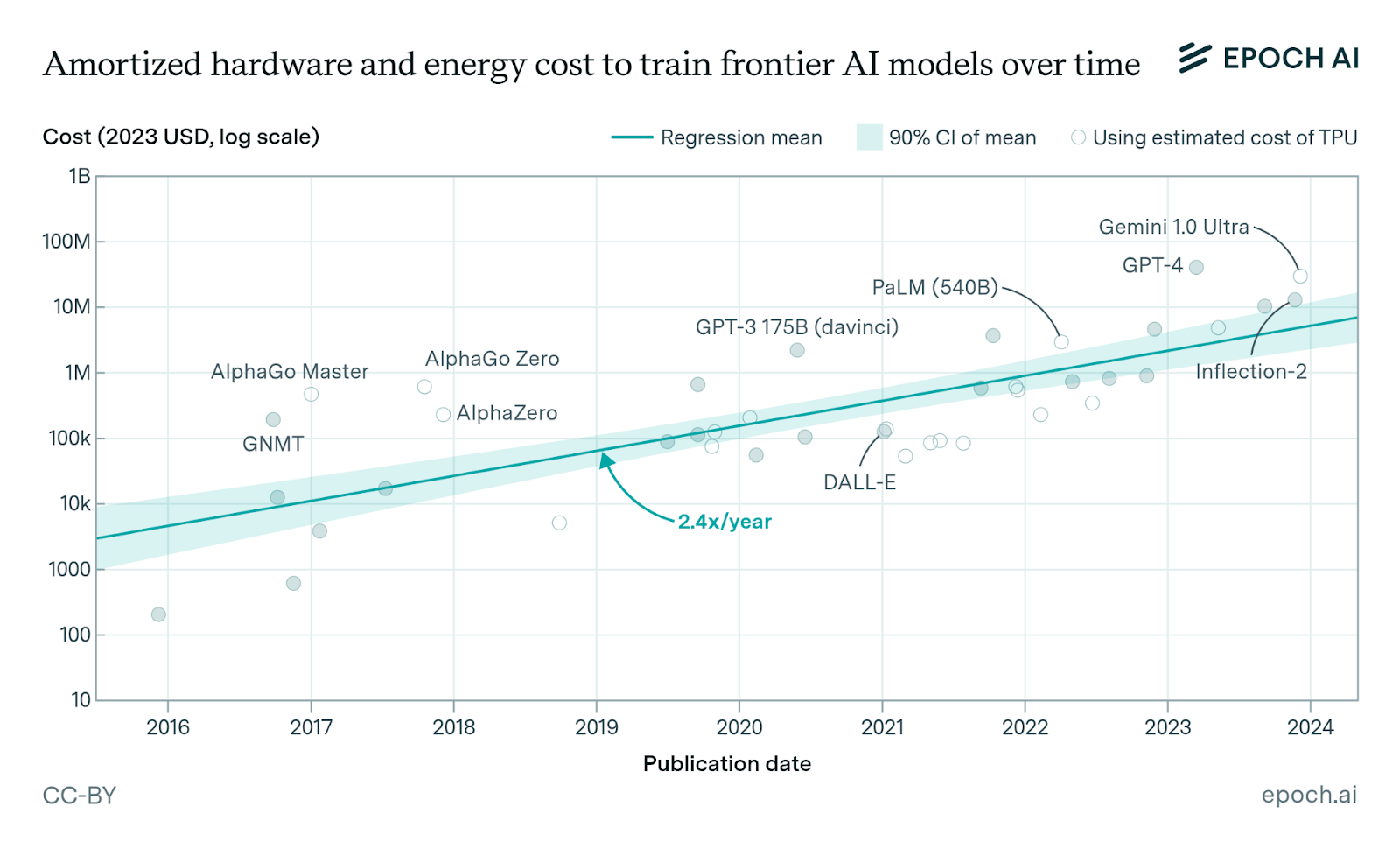
The overall uncertainty band for these bottom-up calculations is roughly 3x, meaning it’s challenging to say exactly when the first billion-dollar runs might be – but assuming the frontier labs will continue to supersede the average, Dario is likely not far off.
Given the enormity of the capex outlays for producing these models, upfront costs and hardware amortization are critical inputs to this ecosystem’s evolution. Frontier labs that own compute infrastructure can double-dip by using the same hardware to both train the models and serve the deployed models to users at inference time, lowering their total operational expenses. The upfront capital required for model development has exploded from $10K in 2016 to upwards of $500M today. This has posed a substantial barrier to emerging players.
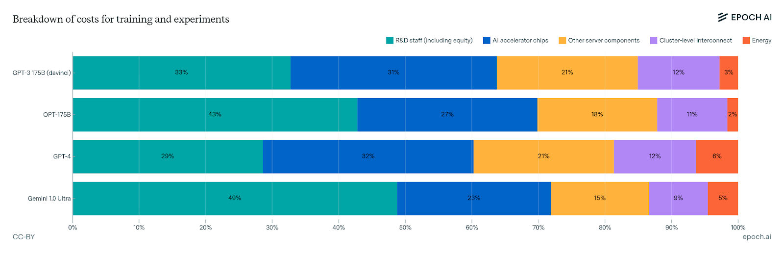
The Epoch AI team also provided a more granular breakdown of pretraining costs to include energy and labor. Broadly, amortized capex and energy comprise 50-70% of LLM development costs while R&D fills out the remaining 30-50%. Within capex, ~46% stems from AI accelerator chips, ~30% from overall server infrastructure, ~18% from cluster-level interconnects, and ~6% from energy, as illustrated below.
The sheer cost of pretraining frontier models makes it difficult for labs to run several large-scale experiments in parallel, meaning researchers have to carefully choose which problems to tackle, what approaches to try at scale, and how to effectively allocate resources during this process. A failed training epoch can cost millions (and soon billions) of dollars, making it more and more critical to understand fundamental pretraining scaling laws and their impact on downstream performance.
How Does Scaled Pretraining Impact Validation Loss?
We’ve established that frontier LLMs are incredibly expensive to train, costing upwards of $500 million and increasing at a rate of 2.4x per year. The next question becomes – what are we getting for it?
We’ll first focus on upstream LLM performance, which is generally called cross-entropy loss or validation loss. In language modeling, this metric quantifies how well the model predicts the next token (e.g., word). Larger losses mean bigger differences between the predicted and actual next token and vice versa.
For years, researchers have sought to understand how increased resource usage during training reduces validation loss. This has given rise to the field’s scaling laws. Here, scale is a function of the number of model parameters/weights (N), the dataset size used for pretraining (D), and the total compute resources (C). Throughout the rest of this section, we highlight some of the seminal advancements made in scaling law optimizations and how they have continuously built on each other’s insights into efficient scaling over time.
Hestness et al. (Baidu)
In 2017, Hestness et al. published one of the first reports of LLM scaling laws across several data regimes including machine translation, language modeling, image processing, and speech recognition. They demonstrated that language model performance improves in a predictable power-law pattern as you scale the model or dataset size.
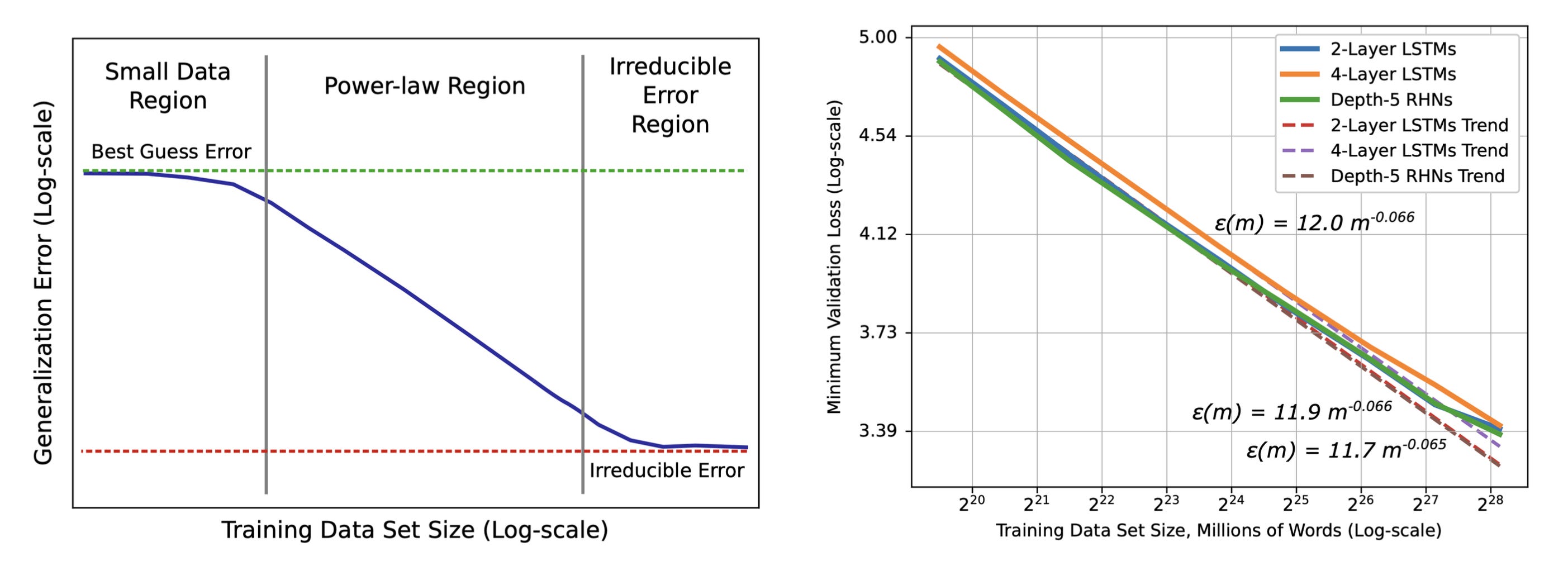
Importantly, optimal model size scales sub-linearly with data size – as you scale up the size of your training dataset (D), you don’t need to increase the number of model parameters (N) at the same rate to keep improving performance. These results laid the groundwork as one of the first blueprints for model developers on how to predict and scale LLM pretraining to maximize accuracy.
Kaplan et al. (OpenAI)
A few years later in 2020, Kaplan et al. expanded on Baidu’s initial scaling laws in two important ways. First, Kaplan et al. used a more modern transformer, attention-based architecture compared to Baidu’s earlier 2- and 4-layer LSTMs (i.e., a common model architecture prior to transformers). Second, they extended the relationships between parameter count, data size, and validation loss to show how compute constraints shape the optimal balance between these factors.
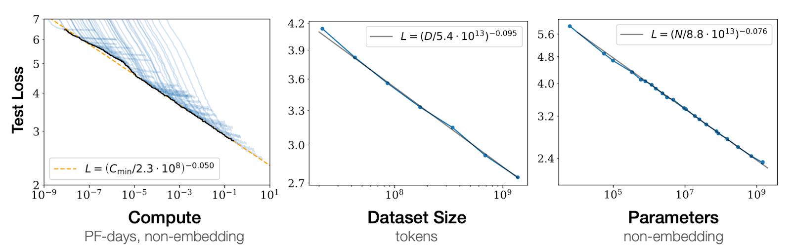
The above plots capture univariate relationships amongst these three parameters. Scaling compute, dataset size, or number of parameters results in a smooth power-law improvement in loss, provided that the other two variables are held constant and not limiting. Kaplan et al. noted that in practice, all three variables can be toggled – necessitating a deeper, multivariate analysis.
The group created plots showing (a) how a fixed set of model sizes (~400K to 708M) trained on a 4-log range of data improves loss as well as (b) how a continuum of model sizes (1M to 100M) trained across a 3-log range of compute (measured in training steps (S)) improves loss.
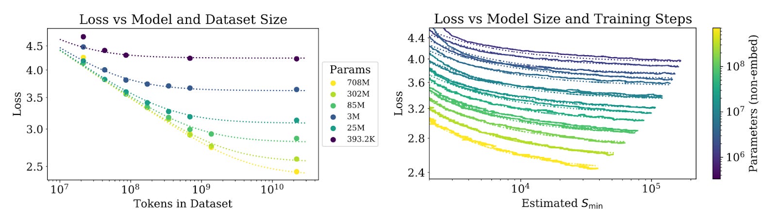
On the left, we can see that larger models have a better capacity to reduce loss when trained on increasingly more data, though with diminishing returns for all the tested model sizes. Using the coefficients from these plots, Kaplan scaling laws suggest that if we increase model size by 8x, we should only increase dataset size by 5x for efficient scaling.
On the right, we can see that for all model sizes, greater compute resources result in an improved loss. Using the data from this second experiment, Kaplan et al. computed the minimal computation budget to achieve an arbitrary loss. They found that given a 10x larger compute budget, the optimal resource allocation suggests scaling model size by 5.5x and data by 1.8x to achieve a maximal loss improvement.
Hoffmann et al. (DeepMind)
Kaplan scaling laws remained state-of-the-art until ~2022, when Hoffmann et al. published a new compute-optimal scaling framework called Chinchilla. The headline here is that Kaplan scaling results in models that are under-trained (i.e., models had too many parameters and not enough training data), while Chinchilla suggests you should use many more data tokens and a smaller model than previously thought. Hoffmann et al. posited that Kaplan et al. came to this conclusion because they didn’t train large enough models and that they used a suboptimal fixed learning rate schedule.
During pretraining, an LLM repeatedly sees small batches of text from its training dataset. For each batch, it predicts the next token, compares that prediction to the actual token, and computes a loss. Based on the magnitude of that loss, the model updates its weights, either by a small or large amount. This process is called a training step and the rate by which the model weights are updated is the learning rate schedule.
Smaller adjustments to the weights can make training more stable, but requires a longer time to converge the model to its final state. Larger adjustments may accelerate learning, but there is a risk of overshooting, leading to model instability and overall poor model performance.
Kaplan et al. used the same cosine learning-rate schedule for every model and dataset size – small updates at the start, large in the middle, and small again at the end. But a cosine schedule only works if you train for the full dataset it was designed for.
Hoffmann et al. argued that when you use a cosine schedule designed for a large dataset on smaller datasets, the training stops early while the learning rate is still high. The smaller models never get to the final low-rate “settling” phase, meaning the weights never converge to optimal performance. This likely altered Kaplan’s conclusions about how to effectively make trade-offs between model and dataset size.
In the Hoffmann et al. paper, the authors trained across a fixed range of model sizes (75M to 10B) and varied the number of training tokens, measuring the loss at several steps throughout the pretraining process. To overcome limitations from the Kaplan et al. paper, they used four different learning rate schedules for each model size. They then computed the model size and training token count that led to the lowest validation loss at each FLOP budget.
As shown below, we can see that all model sizes and dataset permutations result in a quickly improving loss that starts to plateau with higher compute. Diminishing returns occur first with smaller models and later with larger models — the latter being able to access regions of much better absolute loss (e.g., ~2.0 for 10B parameters).
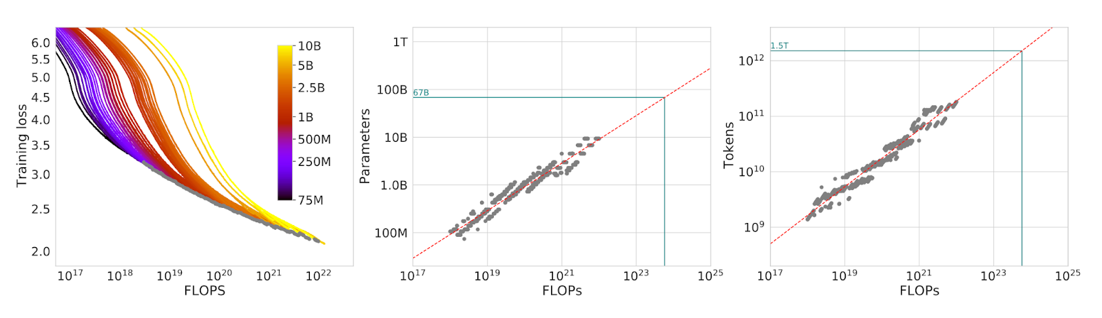
Critically, the Chinchilla-optimal scaling framework arises from increasing pretraining tokens and model parameters at an optimal ratio of 20:1. For reference, GPT-3’s largest model was trained in the Kaplan era with ~1.7 tokens/parameter.
Sardana et al. (Databricks)
In an attempt to reconcile the scaling laws from Kaplan et al. and Hoffmann et al., Sardana et al. published a paper at last year’s ICML with a careful eye toward model scaling from a cost-economic standpoint. The main takeaway was that if a company expects a frontier model to have a high level of inference demand, it’s more economical to train a smaller model with more data and compute until the desired performance is reached. This is because smaller models will require less compute to inference compared to larger models, independent of how much compute was used to train the model in the first place.
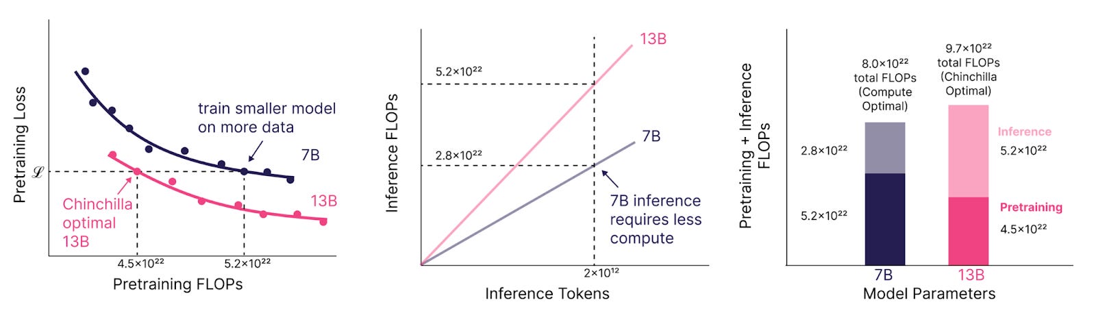
While pretraining this smaller 7B model is Chinchilla-suboptimal (and more expensive), the smaller model is cheaper to run at inference, lowering the operational expenses associated with serving the model to customers. Comparing a 7B and 13B parameter LLM and 2T tokens of inference demand over the life cycle of the model, you can save ~17% (1.7 x 10^22 FLOPs) in compute. For frontier models, that can mean millions of dollars in total savings.
Using this insight, the group at Databricks generated a series of plots that can assist with resource allocation decisions.
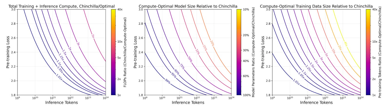
On the left plot, if we wanted to train to a loss of 2.4 and we expect a lifetime model inference demand of 10^12 tokens, we land on the 2x FLOPs ratio band – meaning that a Chinchilla-optimal model would actually cost 2x more than if we were to overtrain a smaller model.
In the middle plot, for the same criteria, we can see that the intersect lands on the 33% band – meaning that a compute-optimal model would have 33% of the parameters of a Chinchilla-optimal model.
On the right plot, the intersect lands on the 5x band – meaning that the ratio of pretraining tokens to parameters should be 5x larger than that of a Chinchilla-optimal model. Roughly 100 training tokens per parameter.
The field has seen this ratio explode in the last couple of years as it has become more popular to train models beyond the 20x Chinchilla scale to optimize for inference costs. For example, Llama-3-70B was trained on over 200 tokens per parameter.
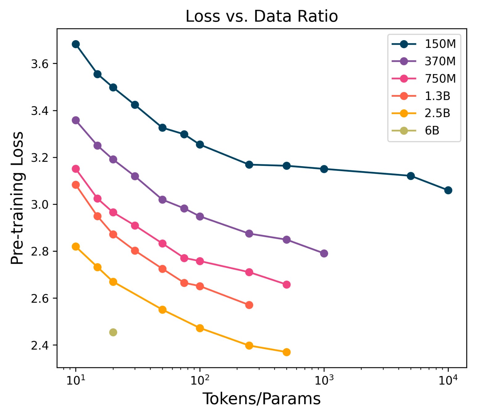
Sardana et al. formalized this trend to show that small models can improve their pretraining loss well beyond the Chinchilla-optimal envelope – even out to 10,000x tokens/parameter. However, they do so at an exponentially decaying efficiency. In the log-scale plot, we can see that the training token-parameter ratio must increase exponentially to maintain a linear improvement in loss. This is true across model scales and poses a significant issue given that we may be running out of the world’s high-quality data.
Can Scaling Dataset Quality Offset Limited Data Quantity?
The pretraining scaling laws developed over the past few years make one thing clear: abundant data is essential for building better, more efficient LLMs. But these studies have largely sidestepped a key question. Can data quality also bend these scaling curves to further optimize model performance in a resource-constrained environment?
The answer seems to be yes – models are what they eat and cooking up Michelin-star data is likely going to be a key consideration for future development.
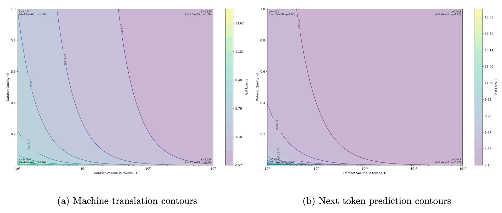
Subramanyam et al. demonstrate this concept well by extending the Chinchilla framework to include a data quality score (Q) and assessing the relationships between model size, dataset size, data quality, and pretraining loss. Here, Q can be thought of as the fraction of high-quality data in the dataset, where high quality refers to uncorrupted, non-redundant text data.
The authors show a clear trend where reduced data quality leads to increased test loss. Interestingly, for tasks like next-token prediction, scaling dataset size from 0.1-10B reduces the model’s reliance on high-quality data. In other words, moderate degradation in data quality can often be offset by training on more total data. Nonetheless, introducing higher-quality data during training is still a relevant knob to increase performance in smaller models.
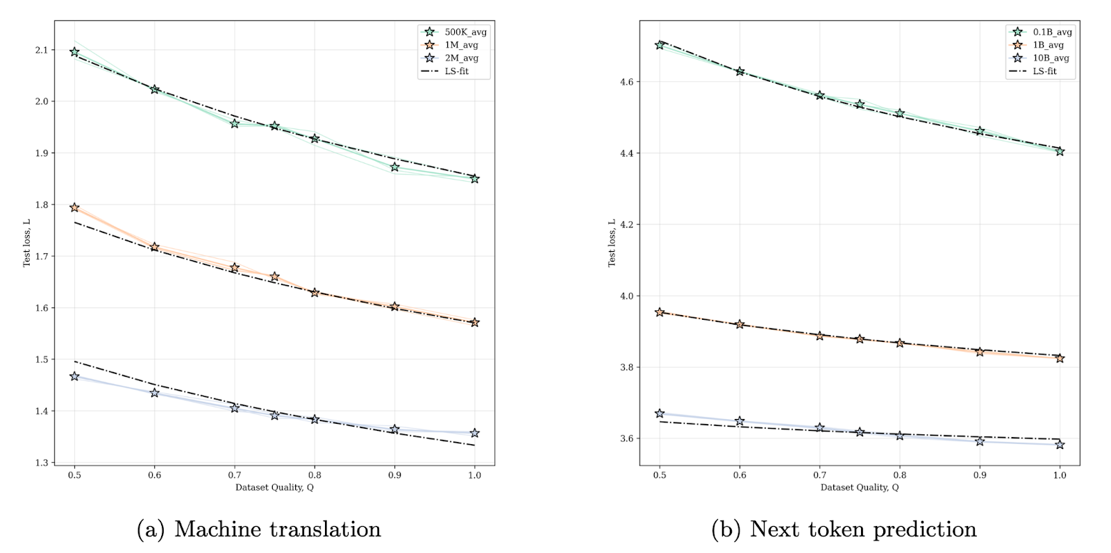
The authors also show that you can get away with training on less data – while still achieving the same test loss – by increasing data quality.
Given these scaling laws, there is a clear need for extracting the highest value per token out of proprietary datasets. In sectors that generate a significant amount of proprietary unstructured data (e.g., customer support centers with billions of call transcripts or insurance providers with historical unlabeled text claims), organizations often have more unlabeled data than they could ever reliably use given compute and cost limitations. As a result, they typically rely on random sampling of their datasets, which significantly limits training efficiency and final model performance.
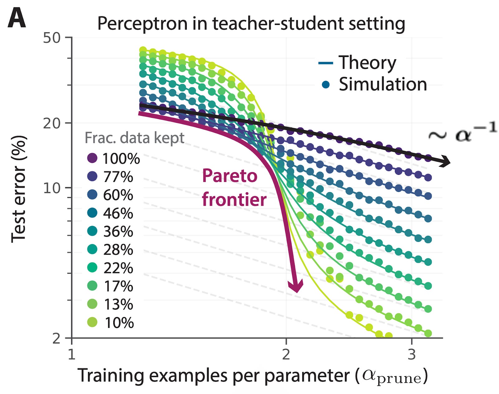
Data curation companies like DatologyAI have developed custom data pruning strategies (e.g., deduplication, model-based filtering, augmentation with synthetic data) to create these high-quality training datasets.
By tiling across pruning fractions, they can experimentally identify the best achievable error across all pruning fractions at each dataset size (i.e., the Pareto front). Notably, the slope of the Pareto front (red) is steeper than the baseline power law scaling (black/purple) when 100% of data is kept in the training set. This illustrates that prioritizing higher-quality training data can result in better-performing models – even though that may mean training on less total data.
Which LLM Benchmarks are Most Common and Useful?
Most of the scaling law data presented so far has focused on validation or test loss as the key optimization metric. However, validation loss is far removed from industrially-relevant tasks and the benchmarks aimed at mimicking them.
LLM benchmarks can be crudely subdivided into a few categories – public, private, and personal benchmarks – that are often scattered across domains like language, math, chatbot assistance, coding, and tool/function calling. Each has its own trade-offs, which complicates unbiased evaluation of models and can often limit interpretability of results.
Public benchmarks (e.g., MMLU, MATH, HumanEval) openly publish their datasets, test suites, and scoring rules, ensuring a level of transparency and standardization across model comparisons. But they can also suffer significantly from data leakage and overfitting (i.e., models seeing test data during training and memorizing benchmarks instead of learning general skills).
Private benchmarks – often developed by frontier labs – offer company-specific evaluations that are resistant to memorization and web exposure, but cannot be easily reproduced and compared across labs.
Personal benchmarks are more vibes-based evals created by each user’s unique interests and work priorities. As a result of their hyper-personalization, these benchmarks may not be useful to the community at large but will likely become more meaningful to users as frontier models continue to become more ingrained in our personal data and applications.
During the formative years of pretraining, early public benchmarks like MMLU (general reasoning) and HumanEval (coding) were popular, but are quickly becoming obsolete. Modern LLMs have become so performant that these more trivial benchmarks are effectively saturated, making them poor barometers for sustained model improvement.
Today, some of the most common benchmarks for frontier LLMs are GPQA Diamond, AIME, and SWE Bench. These evaluate quality and reliability across graduate-level science, Olympiad-level high school math problems, and the ability to resolve real GitHub issues using agentic capabilities, respectively.
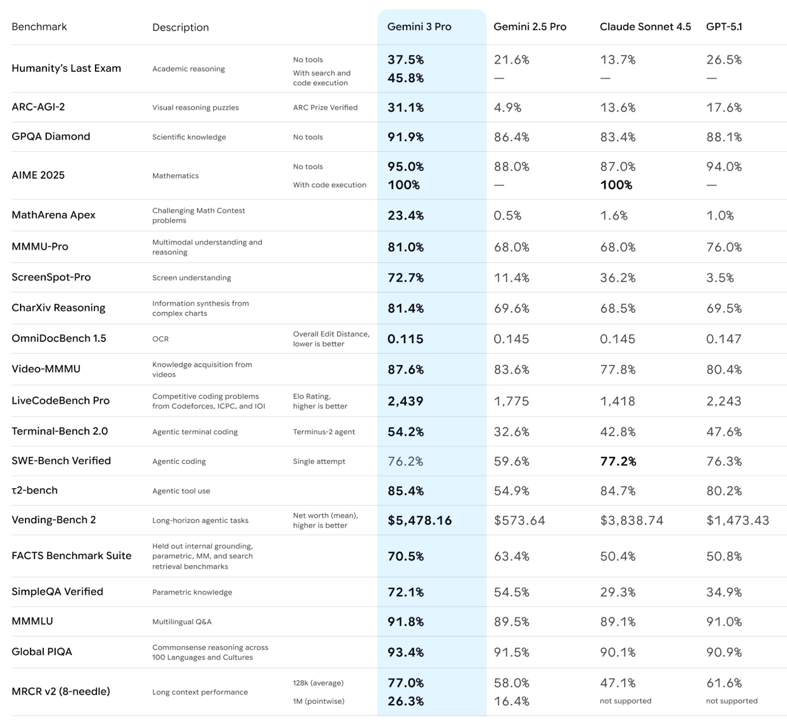
As competition for topping benchmark leaderboards intensifies, frontier labs often publish a laundry list of these benchmark scores comparing their latest models to each other. See the most recent Gemini-3, Claude Opus 4.5, and DeepSeek-V3.2 launch materials. Given the diversity of metrics, it can be hard to quantify the overall capability of the models by simply looking at each benchmark in a list – especially how they change over time.
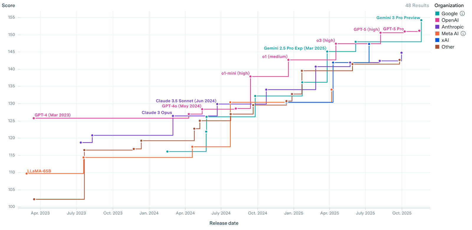
Epoch AI aimed to simplify model comparison by publishing their own Epoch Capabilities Index (ECI), an aggregation of 39 distinct benchmarks into a single score weighted by relative difficulty. Indexes like these provide a more holistic view of model performance and may be more robust to outlier capabilities of one model versus another.
But the ultimate unanswered question is whether any of these benchmarks actually predict any real-world value. While the “dollar per benchmark score” is often unclear, a few studies have attempted to map model improvements directly to labor costs.
For example, Windsurf’s software engineering coding model SWE-1.5 achieved comparable performance to Claude Sonnet 4.5 on SWE Bench, but at 13x the speed. They estimated this speed boost results in a monthly savings of $3-10k in developer time for a 5-person team.
These types of direct benchmark-to-dollars-saved mappings add critical credibility to these scores and should be prioritized as we continue to push these models into the workforce.
Is Validation Loss Predictive of Downstream Benchmark Performance?
So far, we’ve described how scaling pretraining has resulted in predictable, albeit resource-intensive, improvements in upstream validation loss (i.e., next-token prediction). But does reduction in validation loss successfully predict improvement in downstream benchmark performance?
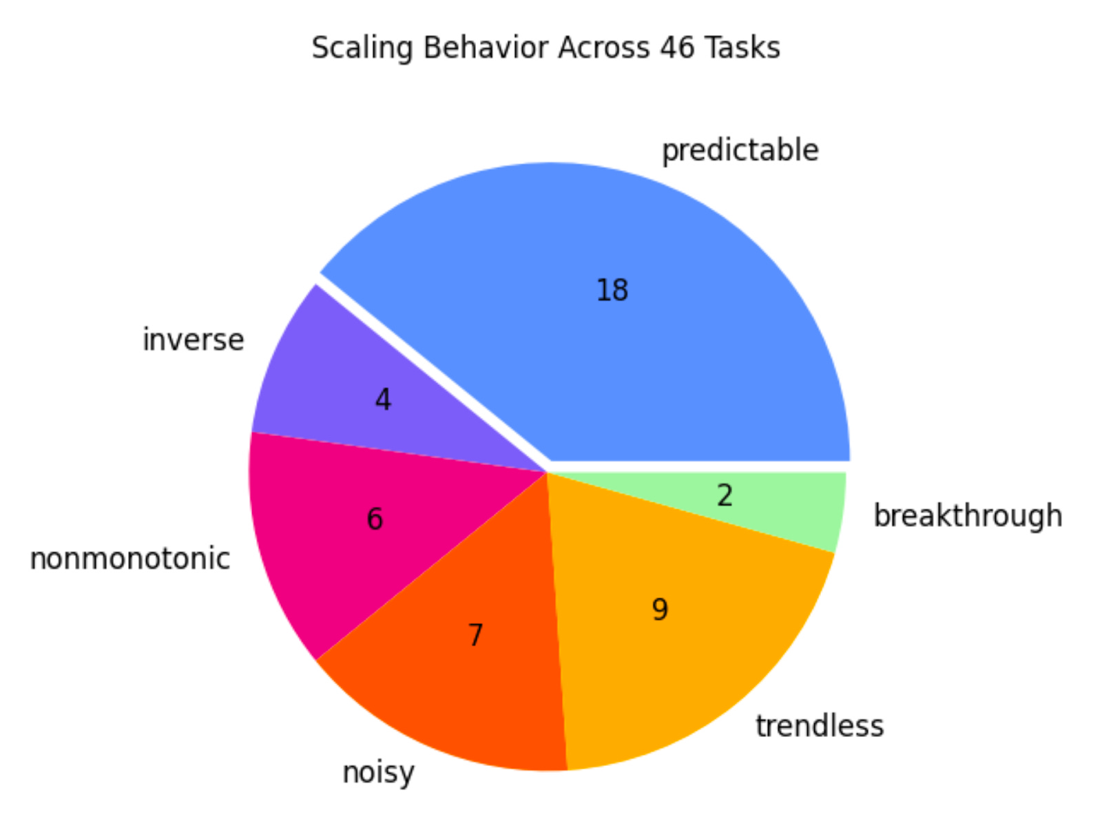
This summer, researchers at Prescient and NYU ran an experiment that produced a surprising result. They found that of 46 common downstream LLM benchmarks, only 39% exhibit predictable improvements when validation loss is reduced. These results are broken down into categories within the pie chart below, alongside examples of what each of these trends (or non-trends) looks like across a set of three different validation datasets.
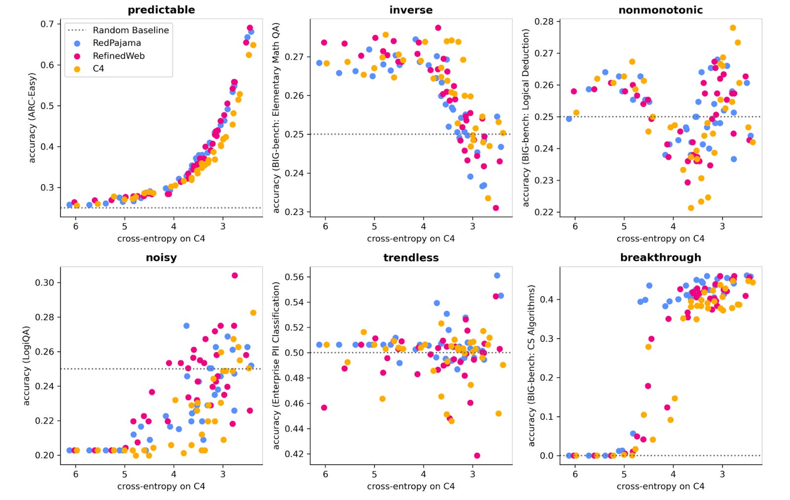
Given these results, it’s clear the predictiveness of pretraining loss for downstream task performance is complicated. There are two interesting categories of model behavior worth exploring more: inverse scaling and breakthrough performance.
Inverse scaling suggests that at some improved loss, downstream task performance passes its optimum and begins to worsen. This can be due to a few different reasons. For example, the pretraining loss is measured on data that simply doesn’t align with the downstream task – a mid-size model might “accidentally” perform well on adversarial multiple-choice questions or logic puzzles because it’s using heuristics to pick the most unusual answer, but larger models index much more to the most common sounding answer which may actually impair model performance in the long run.
While this isn’t the case for every model and every task, it does imply that not all tasks benefit from larger models – there can be substantial product-market fit for smaller models as well. Being able to recognize and exploit this feature can also help providers serve these models much more efficiently.
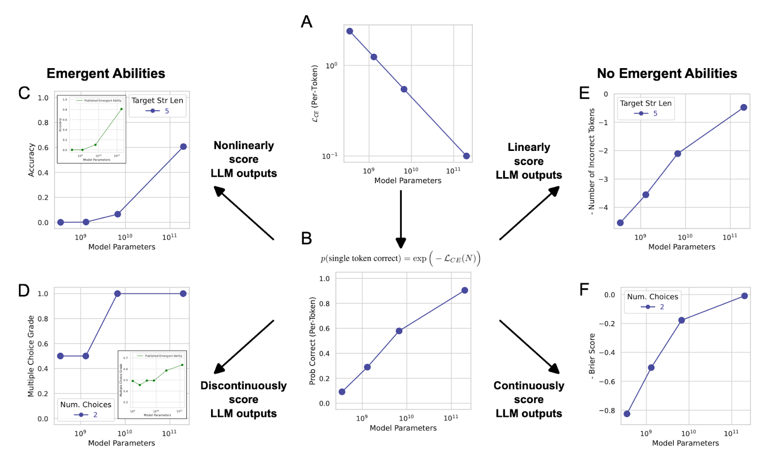
Breakthrough performance (also often referred to as emergence) is the idea that there is a discontinuous step change in benchmark performance at some point during model training. When originally presented, the concept of emergence brought significant concern to the field as downstream performance felt unpredictable. However, elegant work by Schaeffer et al. showcased there may actually be nothing to worry about. Instead, “emergence” is the result of poor experimental design and execution – selecting nonlinear (% accuracy) or discontinuous (multiple choice) metrics with limited data points can trick researchers into mistaking low-resolution graphs for breakthrough results.
What Does the Future Hold for Scaled Pretraining?
We’re in a tricky spot. We now know that scaled pretraining results in improved validation loss and that this improvement in loss can confer a notable downstream benefit. Unfortunately, the benefit is clean in only a minority of cases – which isn’t ideal for large capital allocation decisions and highlights the usage idiosyncrasies that accumulate near the end consumer (e.g., preferring ChatGPT for everyday knowledge questions and reasoning tasks, while using Claude for coding and creative writing).
It’s also clear that achieving improved validation loss solely via pretraining is becoming exponentially more difficult and that the next order-of-magnitude unlocks are running up against some very real physical barriers that could begin to impact frontier LLMs before the end of this decade.
Beyond investors’ willingness to fund AI capex investments in the billion-dollar range, we are running out of training data and running into training length obstacles. Given a lack of infinite compute resources, we need to prioritize where best to allocate resources from one project/model to another.
Epoch AI has written about both of these dynamics. Let’s start with training data.
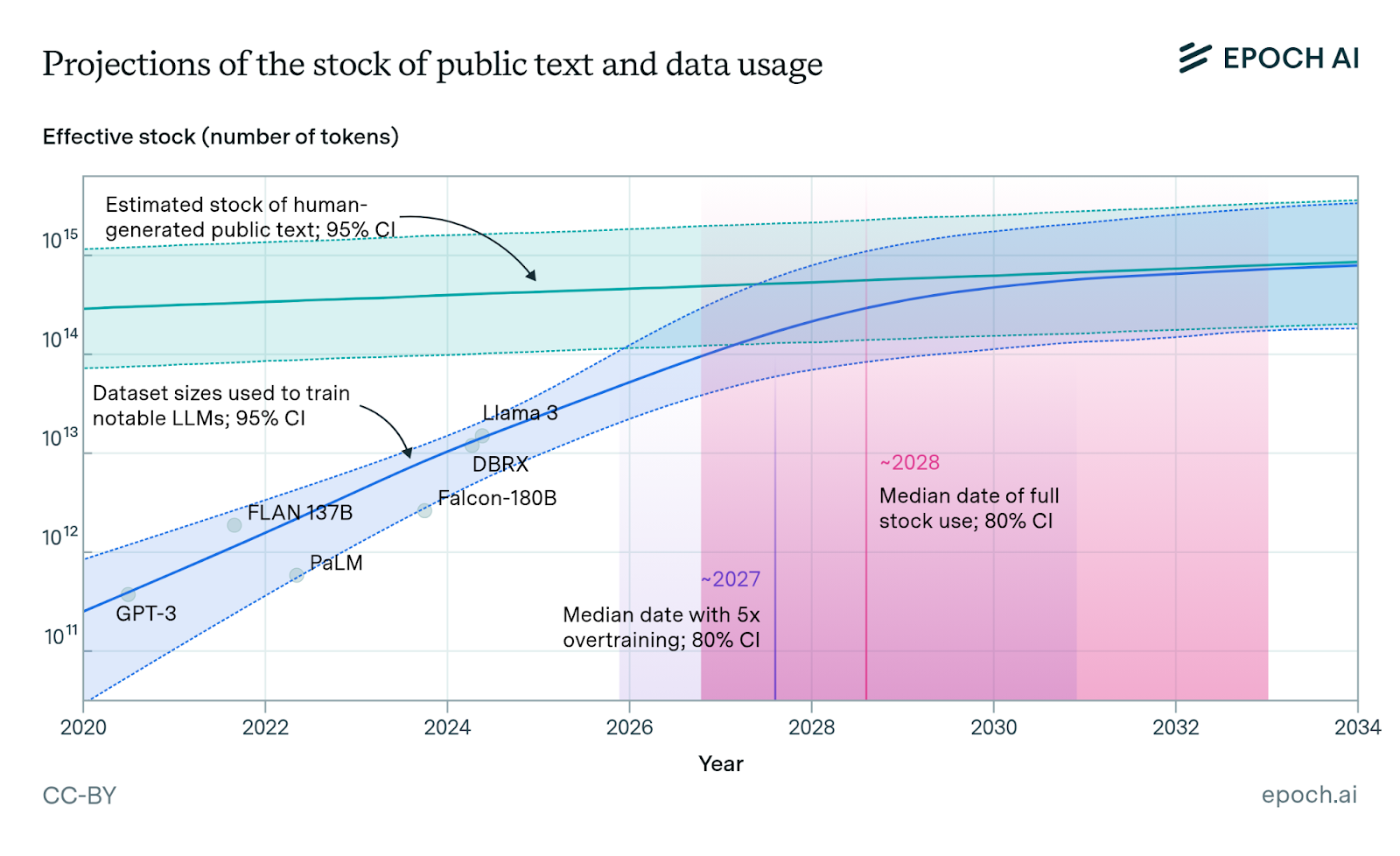
They estimate there are roughly 300T tokens of human-generated, public text available for training AI models. Leveraging our previous insight about overtraining to improve inference-amortization (i.e., post-Chinchilla; fewer parameters and more data), we may exhaust our public training stock near 2028. As discussed above, data quality will continue to become an increasingly important parameter to offset this data scarcity. It should also be noted that other data modalities like images and videos can help supplement this data, but these are often easier to collect and likely not the bottleneck for modern LLMs.
An alternative is incorporating synthetic data (i.e., data produced by advanced LLMs to supplement real-world data). The jury still seems to be out on whether synthetic data can make a large enough dent in our stockpile to sufficiently offset this timeline. The main goal here is to produce novel data that expands the training distribution, rather than just reinforcing data that is already represented in the training dataset. At least for now, synthetic data has been shown to be meaningful in domains such as coding and math, where accuracy of this out-of-distribution data is more easily verifiable. The utility of synthetic data is a topic we will likely expand on in future essays given its potential to upend this data scarcity problem.
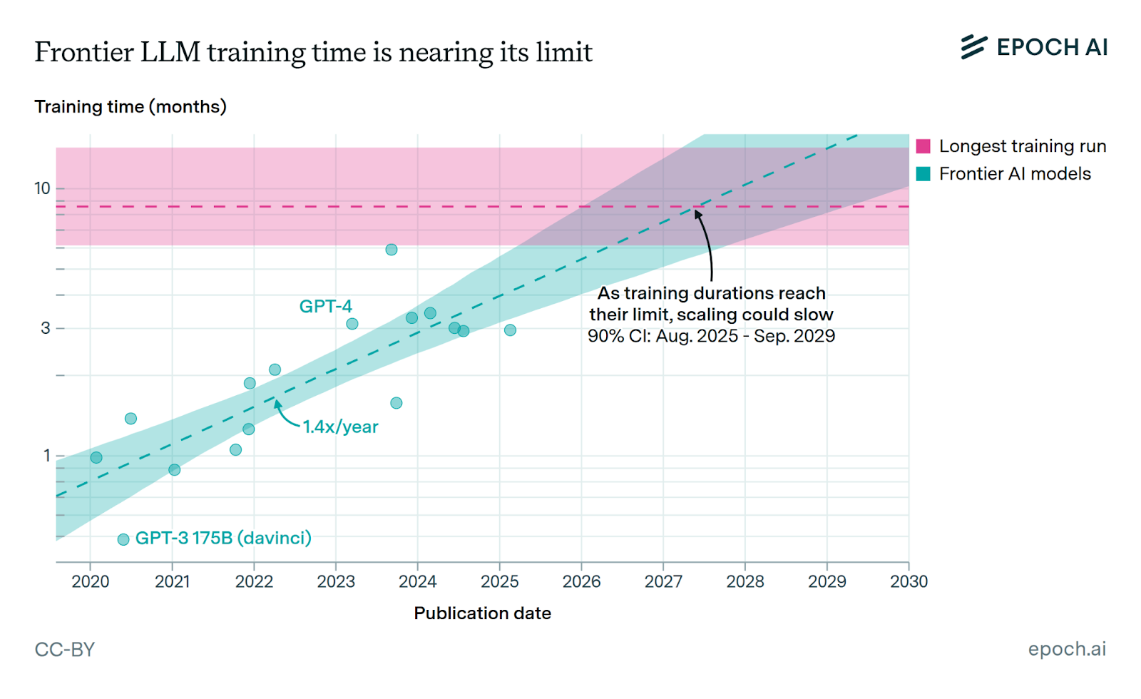
Next, Epoch AI considered obstacles for training length.
Given the rate of hardware and algorithmic improvement, there’s a very real scenario wherein the length of training also becomes a bottleneck. The analysis below predicts training runs can last up to ~9 months before they potentially become inefficient, and we are on pace to meet this milestone by 2027.
To make this more concrete, imagine a scenario where halfway through a 9-month training run, the hardware and algorithms you’re using to train become obsolete. Will this deter frontier labs from making capex investments, effectively freezing the market? Or, will a new wave of ML infrastructure enable the smooth, dynamic reallocation of capex along a training run’s life cycle – effectively building the plane as we fly it? These are still very open questions within the field that will likely define the next era of model training.
Pretraining is Dead(?)
At last year’s NeurIPS conference in Vancouver, former OpenAI co-founder/chief scientist and current Safe Superintelligence founder/CEO, Ilya Sutskever pronounced that “pretraining as we know it will unquestionably end. We’ve achieved peak data and there’ll be no more.”
Given the discussion above, we tend to agree. We can only battle finite data volume/quality, long training timelines, and costly compute/power infrastructure for so long before the pace of model improvements starts to substantially diminish.
While a tantalizing premise, it’s likely safe to say that we cannot simply put the entire universe in distribution to solve our problems. Aside from being impossible from a data and infrastructure perspective, these models would still suffer from rigidity and a constant need to retrain as time advances and new data becomes available.
Fortunately, the field has correctly forecasted these trends and over the last several years has implemented new training techniques to keep performance gains on a steady pace – namely through the introduction of post-training methods and reasoning capabilities.
Reasoning methods aim to teach a model how to logically step through complex problem solving. Their implementation has exploded over the last year with the introduction of OpenAI o1 and DeepSeek R1 – simultaneously unlocking an entirely new scaling regime for model development with few signs of slowing down. This topic will be the focus of our next article.
But does all this mean that pretraining is truly “dead”? Have we overcorrected on pretraining and should we instead shift our focus entirely to optimizing and scaling post-training methods? For several reasons we will continue to explore, we think there is more nuance here, and pretraining will likely remain one of many important knobs to turn in our quest to build more performant and useful AI.
Outstanding deep dive. The Sardana et al. framing around inference-optimized scaling is super clarifying, makes the Llama-3 training choices feel way less arbitrary. Also didnt realize Schaeffer's work basically debunked emergence as just measurement artifacts, thats kinda huge for predicting capabilities.
Baffles me how this piece hasn't got more attention. Really high-quality and palatable for non-technical folks (me).